Matching in R (III): Propensity Scores, Weighting (IPTW) and the Double Robust Estimator

- Propensity Scores 101
- Common Support: We Still Need It, but It’s Easier to Achieve Now
- Propensity Scores Estimation
- Inverse Probability of Treatment Weighting (IPTW)
- Variance of the Estimators: Bootstrap or Analytical Formulas?
- Double Robust Estimator
- Final Remarks: The Most Important Question
- References 📚
Welcome to the final post of this three-part article about Matching estimators in R. First, let’s quickly recap what we’ve seen until now. In the first part we took a look at when we can use these kind of estimators (it’s when the conditional independence assumption holds) and then we dived into some of them, like the Subclassification estimator, the Exact Matching Estimator, and the Approximate Matching Estimator.
Series about Matching
Then, in the second part, we looked at the differences between matching and regression. These mainly boil down to Matching being a non-parametric method (i.e. it doesn’t assume a specific kind of relationship between the variables) that requires common support (that is, having both treated and control units for each set of values of the covariates/confounders). Meanwhile, regression requires us to impose a functional form, but, in return, it can estimate a causal effect even in areas without common support by extrapolating based on the functional form we give to it. This can be good or bad, depending on how accurate is the model specification we’re imposing.
And now, for the last part, we’ll examine another set of relevant Matching topics:
The estimation of propensity scores, a cool way to “collapse” all the confounders in a single scalar number (thus avoiding the curse of dimensionality).
The inverse probability weighting estimator, an estimator that leverages the propensity score to achieve covariate balance by weighting the units according to their probability of being treated.
The double robust estimator, a superb estimator that combines a regression specification with a matching-based model in order to obtain a good estimate even when there is something wrong with one of the two underlying models.
So, let’s look into them!
Propensity Scores 101
The use of Propensity Scores was introduced by the famous economist Donald Rubin in the 70s. As the name hints, these are scores that measure the propensity of receiving the treatment for a given unit, conditional on X (the observable confounders): \(P(D=1|X)\).
Something cool about propensity scores is that they help us avoid the curse of dimensionality. Instead of dealing with the whole feature-space defined by the covariates X, we “collapse” it into a single variable that contains all the relevant information that explains the treatment assignment. In that sense, propensity scores constitute some sort of dimensionality reduction.
The DAG of a propensity score would be something like this:

DAG of the propensity score. Source: Causal Inference - The Mixtape.
As in every DAG, assumptions are expressed by the existence of arrows and also by the absence of them. In particular, note that there is no arrow going directly from X to D. This means we’re assuming that all the effect of confounders X on D is “mediated” by the propensity score. Put another way, we’re saying X can’t provide any extra information about D after conditioning on the propensity score.
Therefore, the propensity score is the only covariate we need to control for to achieve conditional independence and isolate the causal effect of \(D\):
\[ (Y^1, Y^0) \perp D | p(X) \]
This leads to the balancing property of propensity scores: the distribution of the covariates X should be the same for units with the same propensity score, no matter their treatment status:
\[ P(X|D=1, p(X)) = P(X|D=0, p(X)) \]
Common Support: We Still Need It, but It’s Easier to Achieve Now
The propensity score can free us from the curse of dimensionality but not from the need for common support. However, since there are now fewer dimensions, it’s easier to achieve this condition. Instead of needing treatment and control units on each combination of values of X (the original confounders), we just need to have treatment and control units across the propensity score range.
This implies that the observed propensity scores should be strictly between 0 and 1. It also implies that:
To estimate the ATE, the distributions of propensity scores for the treated and untreated units should completely overlap.
If we just want the ATT, the requirement is weaker: we only need the propensity score distribution of the treated to be a subset of the propensity score distribution of the untreated.
There are several ways of checking this. The most basic (but still useful) is to look at the histogram or density plot of \(p(X)\) by treatment status. Here is an example of a density plot where common support doesn’t hold (not even for the ATT).

Note that we don’t need both distributions to look the same (if that was the case, there would be no need for adjustment), but, in order to estimate the ATT, we do need a positive density or weight of the untreated distribution across all the treated group distribution. In the figure above, there is a big chunk in the upper section of the treated group distribution where we can’t find any untreated units, and that’s why we don’t have common support.
A slightly more sophisticated way of doing this is to create bins based on the propensity score and then check that there are observations of both groups in each bin (or, at least, in the bins with treated units, if we just want to estimate the ATT).
Common support checks on the propensity score can be useful as a diagnosis tool even if we use Regression for the estimation itself
Something interesting about these propensity score checks is that they can be useful even if we’re not going to use a Matching-based estimator. If you’re doing regression, you can use them as a diagnosis tool to see how extreme is the covariate imbalance your regression is dealing with, and how much extrapolation it will have to do.
Propensity Scores Estimation
Many of the properties mentioned above (e.g. the balancing property) refer to a theoretical true propensity score. In real life we don’t have access to those but we have to use estimated propensity scores instead.
After estimation, we can check that the balancing property holds by doing a stratification test (Dehejia and Wahba, 2002). This is, looking at bins of our data with similar propensity scores, checking if there are significant differences in their covariates, and thus determining if our propensity scores are “good enough”.
For the estimation itself, we have to fit a model using d (the treatment assignment) as the response variable and X (the covariates/confounders) as the predictors. A common model choice for this step is logistic regression, but we could also use nonparametric machine learning methods such as gradient boosting or random forest1.
ML methods had been shown to perform better at removing covariate imbalance, especially, of course, in contexts of non-linearity and non-additive relationships, so it may be a good idea to go ahead with them if possible.

There are, however, a couple of things to keep in mind when using ML models. The first is to avoid overfitting, which is when our model learns from the noise or sampling variance instead of the true patterns in the data. Secondly, we shouldn’t optimise for accurate prediction of the treatment status but for balancing confounders across treated and untreated groups (which is what the “true” propensity score is supposed to do).
This last point also implies that we shouldn’t include in the propensity score model any variables that are not confounders (i.e. that don’t affect both the treatment status and the outcome) even if they improve the precision of the treatment status prediction2. Including such variables is not only unhelpful but it can even be harmful to our causal inference endeavour as it adds noise to the propensity scores (you can see an example of this here in the book Causal Inference for the Brave and True).
We shouldn’t include in the propensity score model any variables that are not confounders
The good news is that there are several packages in R that optimise for covariate balance when estimating the scores. I took a quick look at them and liked a lot one named twang. This package is being actively developed by the RAND Corporation, has nice methods to measure covariate balance, and supports gbm and xgboost models to carry out the score estimation.
Hands-on example with the twang package
Here we’ll use the data from Lalonde (1986), which is included in the twang package and also appears in the book Causal Inference: The Mixtape. This dataset is very interesting because it combines observations coming from a randomised trial in the mid-70s (experimental data) with observations coming from the general population in the same period (observational data)3.
The treatment in this dataset is a temporary employment program aimed at improving the income and skills of disadvantaged workers. Therefore, if we compare the treated workers against the general population, there will be confounding due to selection bias (the treatment correlates with having low potential outcomes), so the simple difference of means is unsuitable as a treatment effect estimator.
On the other hand, there is a large control donor pool (the comparison group is 2.3 times the size of the treated group). This means that, if the conditional independence assumption holds, we’ll likely be able to estimate the ATT by balancing the covariates through propensity scores.
library(tidyverse)
library(twang)
data(lalonde)
ps_lalonde_gbm <- ps(
# This is D ~ X, a model with the treatment as responde and
# the confounders as predictors
treat ~ age + educ + black + hispan + nodegree +
married + re74 + re75,
data = lalonde,
n.trees = 10000,
interaction.depth = 2,
shrinkage = 0.01,
estimand = "ATT",
stop.method = "ks.max",
n.minobsinnode = 10,
n.keep = 1,
n.grid = 25,
ks.exact = NULL,
verbose = FALSE
)We use twang::ps() for estimating the scores, which in turn invokes gbm for fitting the propensity score model.
Most of the arguments in the function are related to the gbm model itself. Two key arguments are n.trees, the maximum number of iterations, and stop.method, which specifies the covariate balance measure that will be used to choose the optimal number of iterations. For that last argument, we use "ks.max", the maximum KS value (a measure of dissimilarity) among all the pairs of treated-untreated covariates distributions after adjusting for the estimated propensity scores. The lower the ks.max, the higher the balance.
We can use plot() on the output of ps() to visualise the balance measure across the iterations:
plot(ps_lalonde_gbm)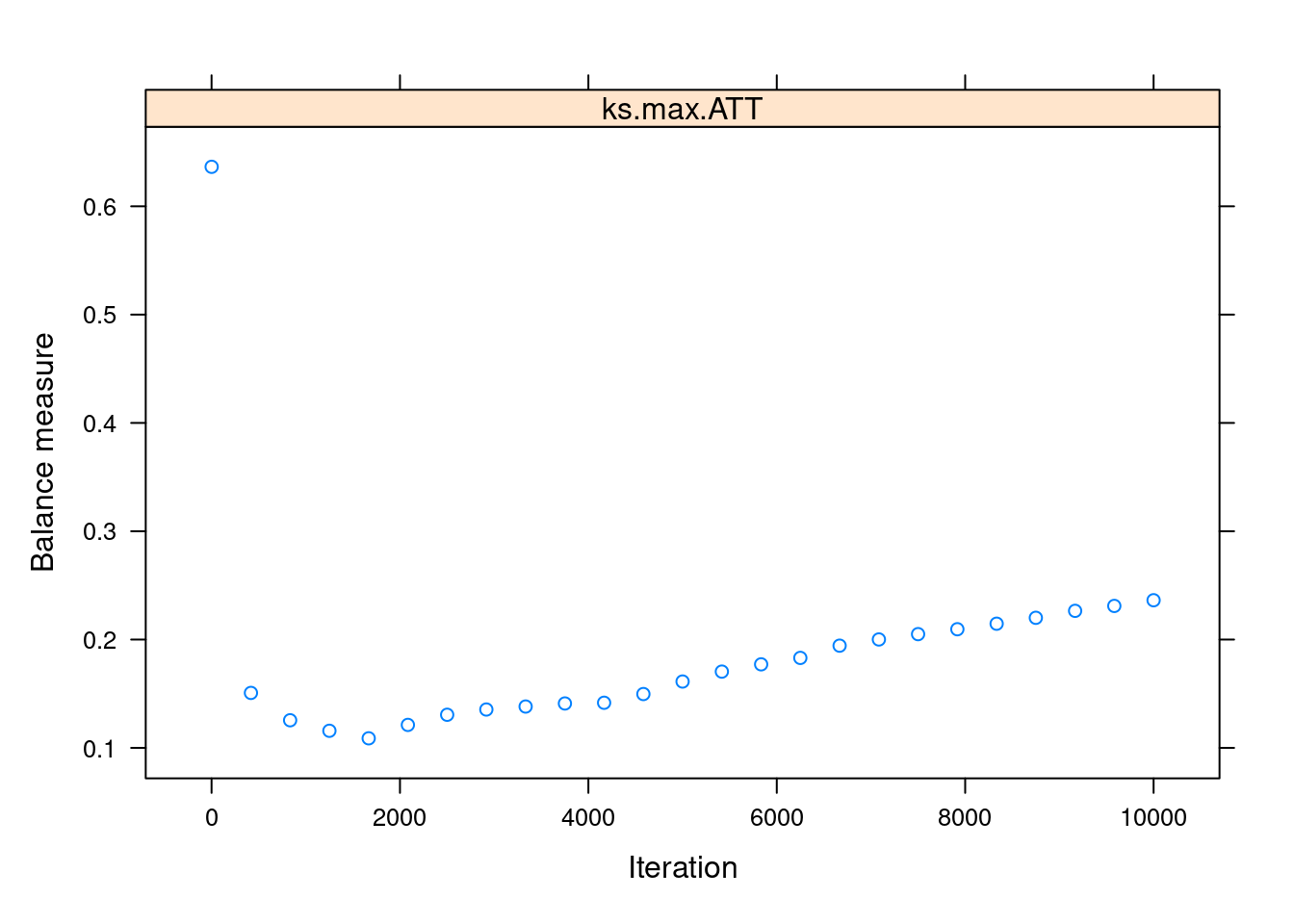
We can see that the balance is maximised somewhere below the 2000th iteration. This “optimal” iteration is the one used for the “final” propensity scores, which are stored under the name ps in the returned object.
head(ps_lalonde_gbm$ps)## ks.max.ATT
## 1 0.6148900
## 2 0.6909022
## 3 0.9234996
## 4 0.9527646
## 5 0.9483888
## 6 0.9527646Inverse Probability of Treatment Weighting (IPTW)
Great! We did it! We estimated the propensity scores! But how do we use them? A common sense and actually popular answer would be to do matching based on them: match each observation with the unit in the donor pool that has the closest propensity score.
Surprisingly, it turns out that matching on the propensity score is a bad idea. A paper from 2018 by King and Nielsen showed several problems with this once well-accepted approach, which may even lead to an increase in the imbalance between groups.
Okay, so matching is out, but then we go back to the first question: how do we use the propensity scores?! Well, there are several valid strategies, but the more recommended one seems to be one called inverse probability of treatment weighting (IPTW).
The key idea of IPWT, as its name says, is to weight the observations based on the probability of them having the opposite treatment status to what they actually have. For example, if a unit has a low propensity score (indicating it was unlikely to be treated) but it was actually treated, then it will receive a high weight and vice-versa: a treated unit with a high propensity score will receive a low weight.
Here the book Causal Inference for the Brave and True nicely sums up why we do this:
If [a treated individual] has a low probability of treatment, that individual looks like the untreated. However, [it] was treated. This must be interesting. We have a treated that looks like the untreated, so we will give that entity a high weight.
After weighting all the units in a group (treated or untreated) we’ll end up with a weighted sample that looks more like the other group. For estimating the ATE, we weight both groups so they both become more similar to each other simultaneously. On the other hand, if we just want the ATE, we weight only the control group in order to make it similar to the unweighted treated group4.
Cool, now that we got the intuition, let’s look at the estimators themselves. First, the ATE estimator, in which we weight both groups simultaneously:
library(rlang)iptw_ate <- function(data,
outcome,
treatment,
prop_score) {
# Renaming the columns for convenience
# (i.e. not using {{ }} afterwards)
data <- data %>%
rename(outcome := {{outcome}},
treatment := {{treatment}},
prop_score := {{prop_score}})
# Estimation itself
data %>%
mutate(iptw = ifelse(treatment == 1,
yes = outcome/prop_score,
no = -outcome/(1-prop_score))) %>%
pull(iptw) %>%
mean()
}Note how the weighting is different (opposite) depending on the unit’s treatment status (makes sense). Also note that, as in the matching estimators from Part I, we subtract the untreated’s weighted outcome because we want the difference between the two groups (treated outcome minus untreated outcome)5.
There is also an ATT version of the estimator:
iptw_att <- function(data,
                     outcome,
                     treatment,
                     prop_score) {

  # Renaming the columns for convenience
  # (i.e. not using {{ }} afterwards)
  data <- data %>%
    rename(outcome := {{outcome}},
           treatment := {{treatment}},
           prop_score := {{prop_score}})

  # Estimation itself
  n_treated <- data %>% filter(treatment == 1) %>% nrow()

  data %>%
    mutate(iptw = ifelse(treatment==1,
                         yes = outcome,
                         no = -outcome*prop_score/(1 - prop_score))) %>%
    pull(iptw) %>%
    sum() %>%
    magrittr::divide_by(n_treated)

}
As we know, the treated units are left untouched for the ATT estimation. However, the weight given to the untreated is slightly different. Why? The Effect by Nick H-K gives us a nice explanation:
The 1/(1−p), which we did before, sort of brings the representation of the untreated group back to neutral, where everyone is counted equally. But we don’t want equal. We want the untreated group to be like the treated group, which means weighting them even more based on how like the treated group they are. And thus p/(1−p), which is more heavily responsive to p than 1/(1−p) is.
Visualizing the IPTW estimator in action with gganimate
To make all of this even clearer, let’s create a gganimate plot that shows how the data is being weighted under the ATT estimator. For this, we’ll attach the propensity scores to the original lalonde dataset and then create two versions of the data:
A weighted dataset using the ATT inverse weighting formula (i.e. weighting the control units to look more like the treated ones but leaving the treated units untouched).
An unweighted dataset, where every unit has
weight == 1.
Then we’ll compute the weighted outcome difference (between treated and untreated) in each dataset. In the first dataset, this difference will be the ATT IPTW estimate, and in the second one, it will just be the “simple difference in outcomes” (the difference we would find in the raw, observational data).
# Attaching the propensity scores to the original dataset
lalonde_w_ps <- lalonde %>%
  dplyr::select(treat, outcome = re78) %>%
  mutate(prop_score = ps_lalonde_gbm$ps[[1]])


lalonde_for_gganimate <-
  # To combine the two datasets we're going to create
  bind_rows(
    # Creating the Dataset with ATT weights
    lalonde_w_ps %>%
      mutate(
        weighting = "ATT",
        weights = ifelse(treat == 1,
                         yes = 1,
                         no = 1 * prop_score / (1 - prop_score))
      ),
    # Unweighted dataset
    lalonde_w_ps %>%
      mutate(weighting = "No weighting (observational)",
             weights = 1)
  ) %>%
  # Creating ordered factors so the legends look nice
  mutate(treat = factor(treat,
                        levels = c(0,1),
                        labels = c("Untreated", "Treated")),
         weighting = factor(weighting,
                            levels = c("No weighting (observational)",
                                       "ATT")))

# Auxiliary summary dataset: means
lalonde_means_gganimate <- lalonde_for_gganimate %>%
  group_by(treat, weighting) %>%
  summarise(mean_outcome = weighted.mean(outcome, weights),
            .groups = "drop")


# Auxiliary summary dataset: estimates
sdo <- function(df) {
  outcome_treat <- df %>%
    filter(treat == "Treated") %>%
    pull(mean_outcome)

  outcome_untreated <- df %>%
    filter(treat == "Untreated") %>%
    pull(mean_outcome)

  outcome_treat - outcome_untreated
}

lalonde_treat_effect <- lalonde_means_gganimate %>%
  group_nest(weighting) %>%
  mutate(sdo = map_dbl(data, sdo)) %>%
  dplyr::select(-data)
library(gganimate)
# requires: install.packages("gifski")
iptw_plot <- ggplot(lalonde_for_gganimate) +
geom_point(aes(prop_score, outcome, color = treat,
size = weights, alpha = weights)) +
geom_hline(data = lalonde_means_gganimate,
aes(yintercept = mean_outcome, color = treat),
size = 1.3,
show.legend = FALSE) +
geom_text(data = lalonde_treat_effect,
aes(label = str_c("Difference Treated minus Control:", round(sdo, 2))),
x =0.5,
y =19500) +
scale_alpha_continuous(range = c(0.2, 0.9),
guide = NULL) +
ylim(c(0, 20000)) +
labs(title = 'Weighting: {closest_state}',
subtitle = "Horizontal line is group average",
x = 'Propensity score',
y = 'Outcome',
color = 'Treatment status',
size = 'Weight') +
# gganimate code
transition_states(
weighting,
transition_length = 2,
state_length = 1
) +
enter_fade() +
exit_shrink() +
ease_aes('sine-in-out')
# Exporting as GIF
animation_obj <- animate(iptw_plot, nframes = 150, fps=35,
height = 400, width = 600, res=110,
renderer = gifski_renderer())
anim_save("iptw.gif", animation_obj)
Handling extreme weights
The previous animation hints at one of the pitfalls of the IPTW method: a disproportionate sensibility to observations in the extremes of the propensity score distribution. Specifically, the weights will approach infinity when treated units have a ps_score approaching 0 or when untreated units have a score approaching 1. This makes the final estimate more vulnerable to sample variance (and what’s more, the weight becomes undefined if the ps_score is exactly 0 for a treated unit or 1 for an untreated unit).
What can we do to mitigate this problem?
A solution commonly seen in papers is performing trimming. This just means dropping out the units with extreme propensity scores values, for example less than 0.05 and more than 0.95. This has the potential drawback of changing our estimand. As in matching, if you discard an important number of units you’re no longer estimating the ATE or the ATT, but an average causal effect on the units that remain in your sample. Depending on the context, this new estimand may or may not be relevant to your audience and stakeholders, so keep that in mind6.
Another alternative is using the ✨normalised IPTW estimator✨, proposed by Hirano and Imbens (2001), which is aimed at better handling the extremes of the propensity score distribution. This estimator normalises the weights based on the sum of the propensity scores in the treated and control groups and thus makes the weights themselves sum to 1 in each group (so we avoid the awkward situation of weights approaching infinity).
Here we have it implemented as code:
iptw_norm_att <- function(data,
                     outcome,
                     treatment,
                     prop_score) {

  # Renaming the columns for convenience
  # (i.e. not using {{ }} afterwards)
  data <- data %>%
    rename(outcome := {{outcome}},
           treatment := {{treatment}},
           prop_score := {{prop_score}})

  # Estimation itself
  treated_section <- data %>%
    filter(treatment == 1) %>%
    summarise(numerator = sum(outcome/prop_score),
              denominator = sum(1/prop_score))

  untreated_section <- data %>%
    filter(treatment == 0) %>%
    summarise(numerator = sum(outcome/(1-prop_score)),
              denominator = sum(1/(1-prop_score)))

  (treated_section$numerator / treated_section$denominator) -
    (untreated_section$numerator / untreated_section$denominator)
}
Alternative IPTW usage: weighted linear regression
As a side note, there are ways to use the propensity scores in a more regression-like fashion. One of them is to just include the propensity score as a control variable in a regression model (y ~ d + ps_score). Another is to pass the inverse probability weights to the weights argument in an lm() call.
In fact, the IPTW estimators we’ve seen until now are equivalent to a simple regression model y ~ d weighted by the corresponding inverse probability weights. It’s easy to conceive extensions to that basic model to account for more complex relationships between the treatment and the outcome.
Variance of the Estimators: Bootstrap or Analytical Formulas?
As we come closer to the end of this series, an element the more stats savvy readers may be missing is standard errors estimation. After all, 99.99% of the time, we’ll get a difference greater than zero between treated and untreated but, without standard errors, we can’t tell if that’s due to a true causal effect or just because of chance (sample variance).
So, how do we compute standard errors for Matching and Inverse Probability Weighting?
An option that may look handy for this is bootstrapping. This procedure consists of obtaining a lot of samples with replacement from the original dataset and then computing the estimate on each of this samples. The result is a sample distribution of estimates, which can be used to estimate the standard deviation of the estimate itself.
And in fact, Bootstrapping is an appropriate way of obtaining standard errors for the IPTW estimator. It also has the advantage of taking into account the uncertainty of the whole process (both the propensity score estimation AND the construction of the weighted samples).
Bootstrap standard errors are often included in packages that perform IPTW, but we can also code them ourselves by passing the data and a bootstrap-compatible function to boot::boot()7. Here is a code example:
library(boot)# This example is an adaptation of this code script shown in The Effect: https://theeffectbook.net/ch-Matching.html?panelset6=r-code7#panelset6_r-code7
iptw_boot <- function(data, index = 1:nrow(data)) {
# Slicing with the bootstrap index
# (this enables the "sampling with replacement")
data <- data %>% slice(index)
# Propensity score estimation
ps_gbm <- ps(
treat ~ age + educ + black + hispan + nodegree +
married + re74 + re75,
data = data,
n.trees = 10000,
interaction.depth = 2,
shrinkage = 0.01,
estimand = "ATT",
stop.method = "ks.max",
n.minobsinnode = 10,
n.keep = 1,
n.grid = 25,
ks.exact = NULL,
verbose = FALSE
)
# Adding the propensity scores to the data
data <- data %>%
mutate(prop_score = ps_lalonde_gbm$ps[[1]]) %>%
rename(outcome = re78)
# IPTW weighting and estimation
treated_section <- data %>%
filter(treat == 1) %>%
summarise(numerator = sum(outcome/prop_score),
denominator = sum(1/prop_score))
untreated_section <- data %>%
filter(treat == 0) %>%
summarise(numerator = sum(outcome/(1-prop_score)),
denominator = sum(1/(1-prop_score)))
(treated_section$numerator / treated_section$denominator) -
(untreated_section$numerator / untreated_section$denominator)
}b <- boot(lalonde, iptw_boot, R = 100)
b##
## ORDINARY NONPARAMETRIC BOOTSTRAP
##
##
## Call:
## boot(data = lalonde, statistic = iptw_boot, R = 100)
##
##
## Bootstrap Statistics :
## original bias std. error
## t1* -632.156 222.9228 1486.774Sadly, bootstrapping can’t be used with the Matching estimators, only with IPTW. The reason is that Matching makes a sharp in/out decision when constructing the matched samples (in contrast to the more gradual weighting done by the IPTW estimator), and this kind of sharp process just doesn’t allow the bootstrap to produce an appropriate sampling distribution8.
Because of that, we have to use analytical formulas to compute the standard errors of our estimates when doing Matching. These expressions can be quite complex and, what’s more, they have different formulations depending on the choices we made regarding the estimation process. Fortunately, most R packages designed for Matching (such as MatchIt) already implement appropriate standard error formulas and report the corresponding SEs in their output. So, if you’re a practitioner like me, it’s better to just stick to these “package-generated” standard errors instead of attempting to compute them manually.
Double Robust Estimator
In Part 2, we saw the strengths and weaknesses of Matching and Regression when adjusting for confounders, along with examples of one of them succeeding in estimating the true causal effect while the other method failed.
But what if we could have the best of both worlds and use an estimator that leverages both Regression and Matching to get the causal effect right most of the time? Sounds pretty cool, right?

Well, that’s precisely what the Double Robust Estimator does. It combines the Regression and the Matching estimations in such a way that we require just one of these methods to be right in order to correctly estimate the treatment effect. Matching right and Regression wrong = we’re fine. Matching wrong and Regression right = we’re fine too.
Of course, not even this super cool estimator can solve our problems if both methods have issues. We need at least one of them to be appropriately specified. Still, it’s a big improvement over using Regression or Matching on their own.
Before showing you a code definition/implementation, note that double-robustness is actually a property that many estimators have, so if you look at the literature, you can find a lot of “double robust estimators”. For now, let’s just look at the one that is shown in Causal Inference for the Brave and True:
# Here I REALLY wanted to parametrise the outcome, treatment and
# covariates variable names, but doing so required to add a lot of
# rlang "black magic" code that made the script harder to
# understand, so what you're seeing here is an implementation
# with the `lalonde` variable names hardcoded.

# TL:DR, you must change the variables names if you
# want to re-use this function with your own data

double_robust_estimator <- function(data,
                        # `index` makes the estimator bootstrap-able
                        index = 1:nrow(data)) {

    data <- data %>% slice(index)

  # Getting the "ingredients" to compute the estimator
  # 1. Propensity scores
  ps_gbm <-  ps(
    # D ~ X
    treat ~ age + educ + black + hispan + nodegree +
      married + re74 + re75,
    data = data,
    n.trees = 10000,
    interaction.depth = 2,
    shrinkage = 0.01,
    estimand = "ATT",
    stop.method = "ks.max",
    n.minobsinnode = 10,
    n.keep = 1,
    n.grid = 25,
    ks.exact = NULL,
    verbose = FALSE
  )

  ps_val <- ps_gbm$ps[[1]]

  # 2. Regression model for treated
  lm_treated <-
    lm(re78 ~ age + educ + black + hispan + nodegree +
      married + re74 + re75,
      data = data %>%
        filter(treat == 1))

  mu1 <- lm_treated$fitted.values

# 3. Regression model for untreated
  lm_untreated <-
    lm(re78 ~ age + educ + black + hispan + nodegree +
         married + re74 + re75,
       data = data %>%
         filter(treat == 0))

  mu0 <- lm_untreated$fitted.vales

  # 4. Outcomes and Treatment status
  outcome <- data$re78
  treatment <- data$treat

  # ✨THE DOUBLE ROBUST ESTIMATOR ✨
  estimator <-
    mean(treatment * (outcome - mu1)/ps_val + mu1) -
      mean((1-treatment)*(outcome - mu0)/(1-ps_val) + mu0)

  estimator
}
# Estimation through bootstrap to get standard errors
# 'dre' stands for Double Robust Estimator
b_dre <- boot(lalonde, double_robust_estimator, R = 100)
b_dre##
## ORDINARY NONPARAMETRIC BOOTSTRAP
##
##
## Call:
## boot(data = lalonde, statistic = double_robust_estimator, R = 100)
##
##
## Bootstrap Statistics :
## WARNING: All values of t1* are NAFinal Remarks: The Most Important Question
We’ve seen a lot of methods and estimators on this three-parter. Sometimes the differences between them are pretty clear, but a lot of times they are much more nuanced. However, if you had to bring only one idea home, I think it should be the Conditional Independence concept we reviewed in the first part (also known as “selection on observables”) and how none of these methods can help you if your data doesn’t meet that assumption.
So, are the confounders directly available in your data as variables you can condition on? THIS is the first-order question you should ask yourself before doing anything else. Only if you have reasons to answer “yes!” to this question you can start weighing if you should perform Regression, Subclassification, Exact Matching, Approximate Matching, Inverse Probability Weighting, or use the Double Robust Estimator.
To check if the “selection on observables” is a credible assumption, you should always summarise your current knowledge about the data generating process in a DAG and then see if this DAG shows a way to close all the backdoors by conditioning on observables9. The package ggdag and its function ggdag_adjustment_set come in handy for this.

If, after doing this, you find that some of your confounders are unobservable, then, as I said before, none of the estimators we’ve just reviewed are appropriate for estimating the causal effect and you’ll have to look for other causal inference methodologies. The good news is that starting with the next blog post, I’ll start reviewing techniques that deal with unobservable confounders, such as Instrumental Variables, Differences in Differences, and Regression discontinuity design, so stay tuned!
References 📚
Causal Inference: The Mixtape - Scott Cunningham. Chapter 5.
Causal Inference for the Brave and True - Matheus Facure Alves. Chapters 11 and 12.
Your feedback is welcome! You can send me comments about this article to my email.
A question you may have here (especially after Part II) is what’s the point of estimating propensity scores using a parametric method like logistic regression when we could just add the covariates as controls to a one-step multiple linear regression instead. After all, one of the benefits of matching-based methods was allowing for non-linear relationships in a nonparametric fashion but we lose that if we use Regression for the propensity score estimation.
I looked for an answer to this and found two key advantages of this approach versus the good ol’ one-step regression (source A, source B).
The first one is that you get common support checks in the second stage. As we saw before, regression extrapolates when there isn’t common support and, what’s worse, it does it quietly. By estimating propensity scores (even with a parametric logistic regression) we gain the chance to look at the histograms/density plots of the scores and use them as a diagnosis tool for how severe is the covariate imbalance. In fact, as it was said before, we have the option of using propensity scores JUST as a diagnosis tool and then dropping them and going ahead with multiple linear regression.
Another benefit is that, due to dimensionality reduction, we save degrees of freedom in the second stage (when the scores are used) by using just a single number (the score) instead of several covariates.↩︎
We’re not trying to win a Kaggle competition, but to approximate \(p(X)\), which, as it notation says, depends on X and nothing else.↩︎
Lalonde used this data to perform a benchmark between several causal inference techniques from that time and the randomised trial (the “gold standard”). Sadly, most methods did just terrible in the paper, but that doesn’t mean they’re useless on their own: it could just be that the assumptions on which they’re based didn’t hold on this data. That’s why, in all the posts about Matching, there has been such a strong emphasis on Conditional Independence, which is the key assumption required for Matching to return a credible estimate.↩︎
Similarly, we could estimate the treatment effect on the untreated (ATU) by weighting only the treated group to make it similar to the unweighted control group.↩︎
An alternative version of the
mutate(iptw = ...line that you may see elsewhere is:iptw = outcome * (treatment - prop_score) / (prop_score * (1 - prop_score))This is actually the same that the
ifelselogic shown before. Whentreatment==1, it collapses tooutcome/prop_score, and whentreatment==0, it simplifies to-outcome/(1-prop_score). IMHO theifelseversion is clearer/more explicit, but just know that if you see this other expression in textbooks, it’s the same thing.↩︎There is an alternative formulation of this technique which consist in capping out the weights at some value (e.g. 20). If a unit ends up with a weight higher than that, we just change its weight to the maximum value. This doesn’t drop observations but introduces bias in the estimate.↩︎
They key thing to remember is that you have to bootstrap all the steps, not just the last part.↩︎
For a more detailed explanation of this, see “On The Failure Of The Bootstrap for Matching Estimators” by Abadie and Imbens (2008).↩︎
If you don’t understand what this last sentence mean, check the Introduction to DAGs blog post.↩︎